Bitcoin-powered genomics

tl;dr things cost money

It’s not news that most bioinformatics resources are short-lived. Websites mentioned in scientific papers go offline at about a rate of 5% per year, and even funding for extremely popular resources like the HapMap Browser can dry up effectively overnight. Indeed, researchers who work on model organisms are currently begging the National Institutes of Health to continue supporting basic informatics infrastructure.

Here, I want to discuss whether this is actually a problem (I’d say yes), one possible solution (paying for things), and one specific toy example of how this could work (a bitcoin-payable interface to the Exome Aggregation Consortium [ExAC] data).

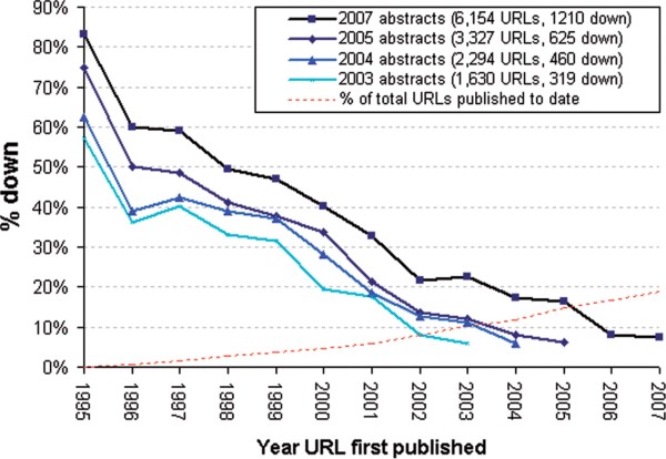
Link rot in the medical literature, from Wren 2008

Is there really a problem, and if so what is it?

There’s a legitimate argument to be made that there’s not really a problem. After all, most papers are rarely cited, so it stands to reason that most software packages or web services are rarely used. And if they’re not used, why should they be supported by grant dollars? Further, the most widely-used resources do in fact get non-trivial levels of funding (the model organism databases discussed above will still get millions of dollars in grants even if the proposed funding cuts go through). So maybe everything is hunky-dory.

However, what this misses is there are a number of important resources that are unlikely to win grants simply because they’re not “innovative” or “novel”, but rather the more mundane “useful”. There are few mechanisms available to sustain projects like this (as has been pointed out many times). More importantly, there is little incentive to actually undertake projects like this–I would probably recommend against an academically-minded student or postdoc taking on a project like “re-implement the HapMap Browser”.

So maybe the problem can be phrased as: we (the scientific community) want two somewhat contradictory things–we want grant money to go to innovation and scientific discovery, and at the same time we want people to maintain resources that work well just the way they are. Any attempt to balance those two things inevitably is going to lead to conflict, and in general I think it’s likely that the former will win out over the latter just on political grounds.

A potential solution: paying for things

Titus Brown alludes to this problem in his post Sustaining the development of research-focused software:

The lesson we can take from the open source world is that, in the absence of a business model, only “community project” software is sustainable in the long term.

The other obvious sustainability model here is of course right there–how about users start paying for things?

The “users paying for things they like” model could even have beneficial consequences beyond simple cash. When The Arabidopsis Information Resource [TAIR] started charging for access, director Eva Huala explained (as paraphrased in Science): “As a bonus…because TAIR doesn’t rely on federal grants, it no longer has to please peer reviewers and can focus instead on what users want”. This comment suggests that perhaps grants are a poor mechanism for funding these types of resources (assuming, of course, that the goal is to make things that users want!).

But charging for access to a database or software has some serious problems–you have to set up an entire billing and sales infrastructure, and even a modest paywall probably reduces your number of users (and thus the utility of your work to the scientific community) by orders of magnitude.

One suggested fix to these problems is “micropayments”–making paywalls so small that they’re not even worth thinking about. Historically this has proved difficult. As Nick Szabo has pointed out, the mental cost of simply thinking about whether something is worth paying for can become the limiting cost in a transaction. Further, interchange fees charged by credit card companies put a lower limit (of at least a few cents) to the size of micropayments that are feasible when using credit cards.

In this context I’ve been intrigued by the work done by the company 21 [1]. Instead of worrying about credit card systems and international wire transfers, they work with Bitcoin, the “money over IP” system. They’ve set up an infrastructure that allows micropayments of a little as a single satoshi (at exchange rates when I wrote this sentence, this is 0.0006 US cents), and software that allows users to trivially get set up with a bit of bitcoin to play with.

How could this type of technology help with the problem I mentioned before?

Toy example: a Bitcoin-payable API for the ExAC database

As a toy example, I threw together a simple bitcoin-payable API for the Exome Aggregation Consortium data. If you’ve installed the 21 software, getting a list of loss-of-function variants in a gene (along with their allele frequencies and a bit of additional information) is then as simple as, for example:

> 21 join
> 21 buy url http://10.244.188.146:5000/lof/PCSK9

Alternatively the API can be called and paid for using the 21 python library. Each API call costs 1000 satoshis (around half a cent), and I’ve implemented endpoints that pull out all annotated variants in a gene as well as all loss-of-function variants (again, this is just a toy example).

All of this is running on an Amazon EC2 micro instance, which will set you back something like $75/year. If the ExAC Browser gets a couple million page views a year, then charging 1/50th of a cent per page view (about 75 satoshis) could cover a few instances, or 1 cent per page view would net $20k, enough for basic electricity plus a bit to play with [2]. In principle, Amazon (or some future cloud computing provider) could set up automatic payments in a system like this, such that any resource that earns enough to cover costs might be maintained on long time scales without human intervention.

Of course, the real benefit here is that once bioinformatics resources start paying for themselves, you can start to build on top of them with a bit more assurance that they won’t disappear overnight. A reliable and self-sustaining infrastructure might open up exciting new possibilities.

—

[1] I have no financial relationship with this company. I do own some bitcoin though; by NIH standards I have a “significant financial interest” in the currency.

[2] I suspect there would be social pressure against anyone actually making a profit on something like this, but I personally wouldn’t have any major objections to students making beer money (I suspect this is the order of magnitude that is feasible in most cases) by building useful tools.

What is genetic correlation?

This post is by Graham Coop and Joe Pickrell.

With the availability of genomic data on large cohorts of well-phenotyped individuals, there has been an increased interest in “genetic correlations” between traits. That is, when testing a set of genetic variants for association with two traits, are the effects of these genetic variants on the two traits correlated?

There are now simple, easy-to-use software packages for calculating these genetic correlations (e.g.), and it is clear that many traits show some evidence for genetic correlation. For example, LDL cholesterol and risk of coronary artery disease are genetically correlated (e.g ).

The most obvious interpretation of a genetic correlation is that it arises as a result of pleiotropy [1]–alleles that affect one trait on average also have an effect on a second trait. This interpretation can shed powerful light on the shared genetic basis of phenotypes, and can also allow the dissection of causal relationships among phenotypes (through approaches such as Mendelian randomization).

Increasingly, however, we will be faced with genetic correlations that are complex to understand and may have multiple causal underpinnings: for example, height is genetically correlated to socioeconomic status, and educational attainment is negatively genetically correlated to body mass index.

Often when these genetic correlations are described they are simply referred to as correlations; this avoids the issue of specifying how they arise. In some cases, though, genetic correlations are directly referred to as pleiotropy. However, quantitative geneticists have known for a long time that genetic correlations arise for a variety of related reasons (e.g.). It is tempting to see the genetic correlations found by GWAS approaches as side-stepping these long-discussed issues. Indeed, if done well they can bypass some concerns (e.g. that correlations between phenotypes within families could be driven a shared environment). However, the deeper issue that genetic correlations can arise through multiple mechanisms has not gone away.

In this post, we want to discuss some of the possible interpretations of a genetic correlation. We start with the two most common interpretations (putting aside analysis artifacts like shared population stratification), and then discuss two additional possibilities, rarely directly tested, that merit further investigation.

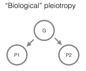
1. “Biological” pleiotropy. In this situation, genetic variants that influence one trait also influence another because of some shared underlying biology. For example, genetic variants that influence age at menarche in women have correlated effects on male pattern baldness. Presumably this is because there are some shared hormonal pathways that influence both of these traits, such that altering these pathways has effects on multiple traits.

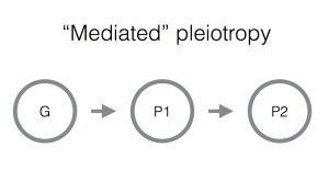
2. “Mediated” pleiotropy. In this situation, one trait is directly causally influenced by another. This of course means that a genetic variant that influences the first phenotype will have knock-on effects on the second. The classic example here is LDL cholesterol and heart disease: these two traits are positively genetically correlated, and it is now widely accepted that this correlation is due to a causal effect of LDL on risk of developing disease. Identifying this situation has important medical implications: since LDL is causal for heart disease, then a non-genetic intervention that influences LDL (for example, a drug or an altered diet) should have an effect on someone’s risk of heart disease.

We note that both forms of pleiotropy may be environmental or culturally mediated. For example, if shorter people are discriminated against in the job market this would generate a genetic correlation between height and socioeconomic status that fits a model of “mediated” pleiotropy.

These two explanations of a genetic correlation are of course plausible. Some other models also seem quite plausible; the relative importance of these different models remains to be seen.

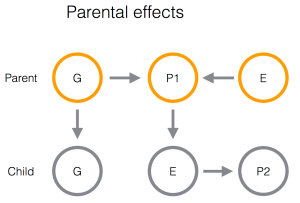
3. Parental effects. For example, imagine that more educated parents pay more attention to the diets of their children, and thus their children have lower rates of obesity. This would be detected in GWAS as a genetic correlation between educational attainment and obesity, though the causal connection between the variant and the two traits is less direct than in the previous two situations. Parental effects can be termed pleiotropy, but importantly the effect is due to the parental genotype, and not that of the child, and so it can be distinguished from within-generation pleiotropy (see below).

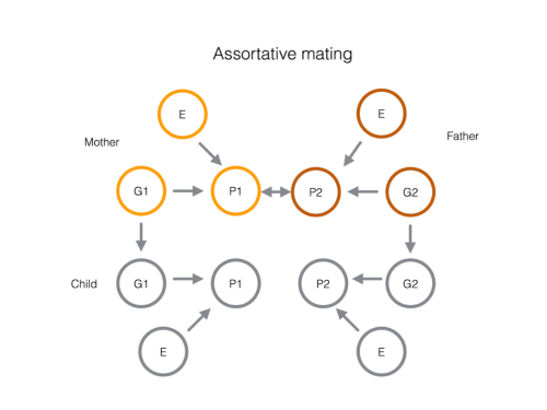
4. Assortative mating. For example, imagine taller individuals tend to marry individuals with higher socioeconomic status. This would induce a genetic correlation between the traits. What is happening is that the alleles that associated with both traits co-occur in the same individuals (the offspring of these assortatively-mating parents).

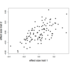
To illustrate this point, we simulated two traits that share no pleiotropic genetic variants in common with 100 unlinked loci each. We simulated cross-trait positive assortative mating for a single generation [2]. We then plotted the effect sizes of the variants causally affecting trait 1 against these perceived affect of these loci on trait 2, as estimated from a sample of 100k children. There is a clear relationship induced by even a single generation of assortative mating.

When alleles that increase both traits are brought together in the offspring this induces a form of linkage disequilibrium (LD) between the loci underlying the same traits (even if the loci are not genetically linked). If this assortative mating continues over multiple generations this LD effect is compounded and builds to an equilibrium level of genetic correlation between the two traits (Gianola 1982).

How can we determine the relative contributions of these latter two causes of genetic correlation? Family studies could help–for example, studies in the UK Biobank have shown that assortative mating contributed to the heritability of height [3], this style of study could be extended to cross-trait comparisons. For example, the polygenic score for each phenotype could be calculated for each parent, and the genetic correlation between parents could be estimated.This would allow for the genetic effect of assortative mating to the assessed. Although we note that even if assortative mating is absent in the parental generation, genetic correlations from previous generations of assortative mating could be present (as they decay through meiotic segregation and recombination).

Similarly, parental effects can be tested by estimating polygenic scores for parent and child (see e.g. Zhang et al.); the contribution of parental and child’s genotype can then be assessed.

Overall, the study of genetic correlations using GWAS data has opened up a number of interesting directions for future work; new methods and analyses are needed to distinguish among these various causes of genetic correlation (and of course, others we have not discussed here).

—

[1] Note that the pleiotropy we see as quantitative geneticists can be mediated through environmental effects. This is simply a statement that alleles affect multiple traits, not that those shared effects have simple “molecular” basis.

[2] Details of the simulation: we simulated 100 genetic variants influencing a trait with 50% narrow-sense heritability. Effect sizes for each locus affecting trait 1 were drawn from a normal distribution, with no effect on trait 2 and the same for the loci affecting trait two. We simulated positive assortative mating with a given correlation coefficient (0.3 in this case) by simulating a male’s phenotype (trait 2) given the female phenotype (trait 1) from the conditional normal, then choosing the male whose value of trait 2 was closest to this. The complete simulation code is available here.

[3] Indeed, while we have explained all of these effects in terms of genetic covariance, they can also contribute to inflating the additive genetic variance contributed by a trait. For example, couples assortatively mate by height, therefore, alleles contributing to tallness tend to be present in taller individuals even more than we would predict from their ‘true’ effect size. Therefore, the effect sizes of alleles may be mildly overestimated by this effect.

Review: Integrating Functional Data to Prioritize Causal Variants in Statistical Fine-Mapping Studies

TL;DR Using functional information improves fine-mapping in genome-wide association studies

I recently reviewed a paper title “Integrating Functional Data to Prioritize Causal Variants in Statistical Fine-Mapping Studies”, which has has now been published. Overall I thought this was a useful contribution that improves on several methodological aspects of fine-mapping in genome-wide association studies.

(NB: none of the points from my actual review are still worth discussing, so the following are my somewhat rambling current thoughts)

Key points

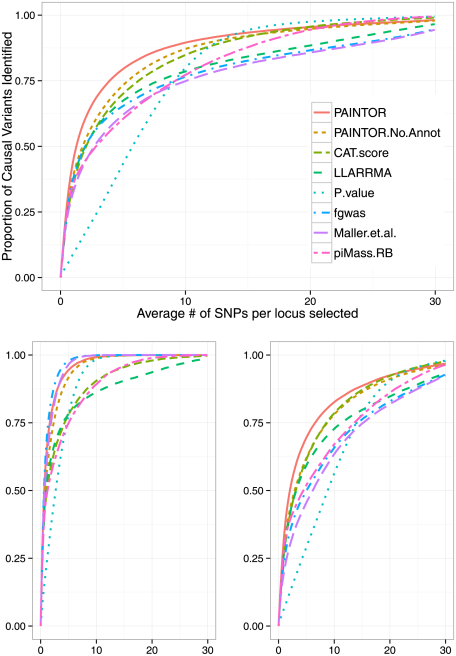
The key to the method here is that 1) it explicitly includes a prior from functional genomic information and 2) it allows for multiple causal SNPs. The figure at the top of this post shows how different methods perform in identifying truly causal SNPs in simulations–in the bottom left is performance in simulations with a single causal variant at a locus, and in the bottom right performance in simulations with multiple causal variants. Perhaps unsurprisingly, methods that explicitly assume a single causal variant (like fgwas, which I wrote) perform best in the former situation, while methods that allow multiple causal variants (like PAINTOR, by these authors) perform best in the latter situation.

Next steps

One thing that I’ve been thinking about is the question: how much do we expect to gain from incorporating functional genomic information into GWAS? In this study, the authors are able to reduce the number of plausible causal variants at a locus by around ~20% using annotations enriched around 5-10X for strong associations (see also a paper from Gusev et al. with similar results); in my own work, I’ve seen that this style of approach also increases the number of identified associations by around 5%. This shows that this line of work is on the right track, but personally, I’d perhaps naively expected this approach to be more powerful. A couple possibilities:

1. Do we have the right functional annotations? One possibility is that we don’t have data from the tissues and experimental conditions that are most relevant to annotate disease-related SNPs–for example, perhaps we need to incorporate maps of transcription factor binding in stimulated immune cells, or from different developmental stages. Some nice work along these lines has been done by Fairfax et al.
2. Do we need to get better at predicting which SNPs in an annotation are important? Another possibility is that we’re doing a poor job of distinguishing SNPs that matter from SNPs that don’t; e.g. two variants could both fall in an annotated transcription factor binding site, but only one might actually influence binding. Important work along these lines has been done by Moyerbrailean et al.

It seems unlikely that there’s going be be a “magic bullet” that works in all situations; rather, it will take progress on each of these points, plus the development of new methods that use all these different sources of information together.

The burden of the “multiple testing burden”

I’ve written before on this site about the way metaphors influence scientists and motivate entire directions of research. I was thinking about this again during talks at the meeting of the American Society for Human Genetics, where I was repeatedly reminded of that albatross hanging around the necks of anyone looking genome-wide for variants that influence disease risk: the “multiple testing burden“.

Over and over again, I was told by speakers that an unfortunate side effect of looking at a whole genome is that there are so many things to look at–as all good statisticians know, we brush our teeth twice a day, floss once, and always correct for multiple comparisons. This correction (requiring more stringent thresholds in a genome-wide study than in a targeted study) is our “burden”.

This rather Puritanical point of view (which has always been a bit odd [1]) has one important upside: it encourages stringent thresholds for calling a “true” association. For example, in GWAS, the heuristic P-value threshold of 5×10^-8 has proved incredibly useful for avoiding follow-up work on false positives.

However, this point of view also has one important downside: it implicitly suggests that the multiple testing “burden” can be “lifted” simply by looking at fewer things! But this makes no sense: taken to the logical extreme, it suggests that a reasonable study design would be to only consider rs78704525 (to randomly choose a SNP) in all future studies. So much burden gone!

So I’d like to replace the idea of the “multiple testing burden” in genomics with something a bit more upbeat. Perhaps a “multiple testing party”. As in: “we collected 1,000 phenotypes and 1,000,000 genotypes on all study participants. Naturally, this required throwing a multiple testing party”. The more the merrier! [2]

—-

[1] As has been pointed out, for example, by one of the first successful genome-wide association studies [WTCCC 2007]:

Classical multiple testing theory in statistics is concerned with the problem of ‘multiple tests’ of a single ‘global’ null hypothesis. This, we would argue, is a problem far removed from that which faces us in genome-wide association studies, where we face the problem of testing ‘multiple hypotheses’ (for a particular disease, one hypothesis for each SNP, or region of correlated SNPs, in the genome) and we thus do not subscribe to the view that one should correct significance levels for the number of tests performed to obtain ‘genome-wide significance levels’.

[2] More seriously, by simultaneously looking at millions of genetic variants and thousands of phenotypes, one can identify systematic biases in the data and potentially correct for them (c.f. Leek et al. 2010), and in principle learn what proportion of variants influence each trait (c.f. Storey 2001). This is not a “burden”, it is actually a huge advantage.

Are parameter estimates from fgwas unbiased?

(Short answer: yes)

In my recent paper describing a hierarchical model for genome-wide association studies, I present estimates of the proportion of GWAS hits for different phenotypes that are driven by non-synonymous variants. A colleague recently wrote to tell me there was some debate in his journal club about whether these estimates (and other such estimates in the paper) are unbiased. I had simply assumed this was the case, so there is no discussion of this point in the paper.

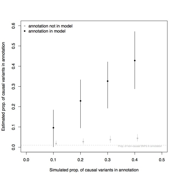
To test whether this intuition is correct, I performed simulations of an association study of a quantitative trait with ~100 causal variants, and I assigned causal variants to a simulated annotation as varying rates (Instead of a detailed description of the simulation methods, I’ve posted my code to GitHub). I then ran fgwas and estimated the proportion of causal variants in that annotation, and then repeated this simulation 100 times. Shown in the Figure above are the range of these estimated proportions in the 100 simulations, excluding the 10 most extreme estimates (the 5 highest estimates and the 5 lowest estimates).

The estimates do appear to be unbiased in these simulations (as well as simulations with a higher baseline rate of non-causal SNPs in the annotation, see here). By contrast, a naive estimator of the fraction of SNPs in the annotation that does not use knowledge about enrichment (in grey) is a severe underestimate.

Review: Geographic population structure analysis of worldwide human populations infers their biogeographical origins

This post is part of an experiment where I will be posting summaries and critiques of the main points of papers I review for journals. Apologies in advance for any misunderstandings and errors on my end; please correct these in the comments.

TL;DR: I have a conceptual disagreement with a paper on learning about the geographic origin of individuals from genetic information.

I recently reviewed a manuscript titled “Geographic population structure analysis of worldwide human populations infers their biogeographical origins”, which has now been published. Overall I found the paper difficult to review because the authors and I have fundamentally different views about what genetic information can tell us about geography. I hope to explain this a bit in this post.

(Side note: some of the authors have started a company called Prosapia Genetics to sell a product based on this paper, but in the paper write “The authors declare no competing financial interests”. This seems to run counter the spirit of these types of disclosures).

(Side note 2: Pseudonymous blogger Dienekes Pontikos notes that the method in this paper is extremely similar to one he developed a few years ago. Regardless of the intentions of the authors, I personally apologize to Dienekes for not noticing his previous work).

The goal of the paper and the associated method

Imagine you had my genome sequence. The goal of this paper is to develop an algorithm to place me on a map–that is, to find the latitude and longitude of my “biogeographical origins”, a concept that I think can be vaguely defined as the geographic location of my ancestors sometime in the recent past (for a European-American, maybe sometime in the last few hundred years prior to the major European migrations to the US)

One way to do this is to imagine the world as a grid (either in 2D or 3D space), and build some model for how the frequencies of genetic variants vary across space. If you had my genotypes at a number of variants, you could then find the best spot for me on this grid. This is the basic idea underlying previous work on this topic, for example in Spatial Ancestry analysis.

The authors of this paper take a different approach. Instead of explicitly modeling geographic variation in the frequencies of alleles, they first perform a clustering analysis on a reference set of individuals with known geographic locations. They then (more or less) find the clusters I fall closest to, and copy over the geographic information from those clusters. That is, if genetically I seem most similar to a reference group of French and German individuals, then they say that my “biogeographic origin” is between France and Germany.

Conceptual issue: This is a paper about genetic clustering, not about geography

Basically, geographic information plays no role in this algorithm except in a post hoc manner. Instead, this is a standard genetic clustering algorithm. This means it has the same limitations as any such algorithm. For example, in the Figure above, imagine a set of reference individuals colored according to their inferred “cluster”. Now imagine matching test individual 1 to those clusters. In this case, it’s simple: individual 1 matches cluster 1, and so copying over the geographic information from cluster 1 to individual 1 seems reasonable. But what about individual 2? This individual doesn’t match any of the reference clusters, so the algorithm can’t do anything with it. If the algorithm were truly learning about geography, this wouldn’t be the case.

As the authors note, a whole host of other limitations come along with this. For example, the authors assume the reference populations can’t have changed geographic locations in the time frame of interest (implying the method is limited to populations with historical records attesting to their residency in a geographic location). That is, imagine that 200 years ago, everyone from one reference village moved 200 km to the west for some reason–this algorithm would place the descendants of that population in the present-day location, rather than the historical location. This is all fine if the goal is genetic clustering, but the authors interpret their algorithm strongly in terms of geography. This leads to something of a tautology: this algorithm can use genetic information to infer geography only if you assume genetic clusters are geographically meaningful*. The utility of the method thus depends on whether this is the case in any particular application.

*The sentence has been edited for clarify

Review: High Resolution Genomic Analysis of Human Mitochondrial RNA Sequence Variation

This post is part of an experiment where I will be posting summaries and critiques of the main points of papers I review for journals. Apologies in advance for any misunderstandings and errors on my end; please correct these in the comments.

TL;DR: A clever analysis of RNA sequencing data identifies natural genetic variation influencing mitochondrial tRNA processing in humans.

I recently reviewed a manuscript titled “High Resolution Genomic Analysis of Human Mitochondrial RNA Sequence Variation”, which has now been published. Overall I thought the paper was creative and surprising; I’d be interested in hearing other folks’ thoughts.

The experiment

The initial goal of this study seems to have been to use RNA-seq to quantify variation in mitochondrial RNA and DNA sequences. The authors sequenced cDNA libraries prepared from mRNA from whole blood in ~700 individuals, and focused specifically on sequencing reads that mapped to the mitochondrial genome. Since each individual in principle inherited a single mitochondrial genome from their mother, there should be essentially no sequence-level variation within individuals (modulo sequencing and mapping artifacts, more on this later).

The authors then did a simple analysis: they looked for positions in the mitochondrial transcriptome where they observed more than a single base in an individual. They identified ~600 such sites (some observed in multiple individuals), which they call “heteroplasmies”. Putting aside potential technical explanations for these sites, heteroplasmies could be due to either 1) variation at the DNA level (e.g. mutations that have occurred in mitochondria of the individual’s blood during their lifetime) or 2) variation at the RNA level (post-transcriptional modifications of RNA through mechanisms like RNA editing).

Main result: A genetic variant in MRPP3 influences processing of mitochondrial tRNAs

At 13 of the heteroplasmic sites, the authors noticed that their data contained multiple alleles (rather than the two you might expect from a new mutation or a simple RNA editing event). They also made an odd observation: 11 of these 13 sites fell in the ninth position of tRNA genes. By reference to what is known about tRNA biology, they argue that the particular patterns of mismatches they observe at these sites are caused by the presence of RNA methylation (which causes the observed mismatches via reverse transcriptase errors).

Under this model, the proportion of non-reference alleles at a site is a quantitative measure of the fraction of mitochondria in an individual that is methylated at the site. The authors reasoned that as a quantitative phenotype, genetic variants influencing methylation levels might be mapped by standard human genetics methods. Shown at the top of the post is a “Manhattan plot” showing the authors’ results from a genome-wide association study of (putative) tRNA methylation in the mitochondria. The result is essentially every human geneticist’s dream: there’s a single strong peak centered on a nonsynonymous SNP in a biologically plausible gene (in this case, MRPP3, a gene involved in processing of mitochondrial tRNAs).

Putting all of this together, is seems that there is variation in mitochondrial tRNA methylation (or some other modification that could cause similar reverse-transcriptase errors) among individuals in a population, and that this variation is partially due to a trans-acting genetic variant of relatively large effect. I found this is quite impressive.

A note of caution regarding estimates of the total number of heteroplasmies

At various points in the paper, the authors include other results that are often interesting but not as important to the main conclusion. One of these that is worth thinking about is the overall number of heteroplasmic sites.

The authors estimate that in their samples, there are around 600 mitochondrial sites that have multiple alleles (note that this is a sum of DNA-level heteroplasmies and RNA-level heteroplasmies). I have a nagging suspicion that this is an overestimate.

The reason for this suspicion is that I’m worried about mapping errors from “nuclear mitochondrial DNA” (AKA Numt) sequences causing false inference of heteroplamies. Examination of some of the reported sites suggests that the alleles of the “heteroplasmies” indeed are consistent with instead being due to mismapping errors from autosomal sequences.

For example, below is a screenshot of the UCSC genome browser surrounding two “heteroplasmic” sites from Supplementary Table 1. I’m showing the sequence of the reference mtDNA (at the top), as well as the sequences of all relevant Numts (using the NumtS Sequence track). As you can see, at the two sites called by the authors, the alternative “allele” at the site matches the sequence of the Numt. My guess is that there is no mitochondrial sequence variation at these two sites, just mis-mapped sequencing reads that originated from the Numts.

It’s unclear how many of the sites identified by the authors are potentially affected by mapping errors (though note none of the 13 used in the mapping experiment described above have any indication of such problems to my eye). For people interested in quantifying the overall extent of the phenomenon observed by the authors, this seems like a potentially important source of error to take into account.

Y-chromosome “Adam” was not necessarily human

Metaphors in science play an important role in communicating results from one field to scientists in other fields and to the general public. In some cases, however, metaphors are so successful and so appealing that they actually obscure rather than enlighten.

In human population genetics, it is a simple fact that all of the Y chromosomes present in the world today can be traced back to a single common ancestor–if you follow my paternal line (my father’s father’s father’s father, and so on) and your paternal line back far enough, eventually they will overlap. At some point, a population geneticist had the clever idea of calling this common ancestor “Adam”. This is a biblical allusion, of course, and it probably was good for a bit of amusement a couple of decades ago. But it’s time to retire this metaphor–not only because it confuses the public (see a nice series of posts by Melissa Wilson Sayres on this topic here) or scientists in other fields–but because it confuses even practicing human population geneticists!

I was reminded of this when reading over a paper by Eran Elhaik, Dan Graur, and colleagues critiquing work on the human Y chromosome phylogeny by Mendez et al. The basic question being debated is: when did the most recent common ancestor (MRCA) of all Y chromosomes exist? Mendez et al. claimed that this Y chromosome was present around 300,000 years ago, and Elhaik et al. claim they arrived at this number incorrectly.

The details of these papers are not relevant for this post. The key thing I want to point out is an underlying assumption, perhaps most clearly expressed by Elhaik et al., who write:

[Mendez et al.] estimated the time to the most recent common ancestor (TMRCA) for the Y tree to be 338,000 years ago (95% CI=237,000–581,000). Such an extraordinarily early estimate contradicts all previous estimates in the literature and is over a 100,000 years older than the earliest fossils of anatomically modern humans. This estimate raises two astonishing possibilities…

The implicit assumption here (the reason Elhaik et al. find the numbers “extraordinarily early” and “astonishing”) is that the individual carrying the most recent common ancestor of all human Y chromosomes (AKA “Adam”) should be an anatomically modern human. Amusingly, Elhaik et al. argue that to claim otherwise is analogous to claiming you have a unicorn in your backyard. But there is simply no reason that “Adam” must be a human. At the top of this post I’ve put a figure showing a hypothetical Y-chromosome genealogy superimposed on a hypothetical human phylogeny. In this (of course hypothetical) example, “Adam” existed well before the diversification of modern humans; this type of scenario is perfectly compatible with basic population genetic theory. From the point of view of population genetics, there is absolutely no reason that the common ancestor of all human Y chromosomes must have existed in an individual that we would identify as “human”.

So why would anyone make this assumption? Note that Elhaik et al. made a YouTube video describing their results; this video leads with a bit of religious iconography. It seems plausible that by calling the most recent common ancestor of all Y chromosomes “Adam”, population geneticists have confused themselves into thinking that “he” must have been human.